When a Model Is Wrong, the Cause May Not Be the Model

An unexpected prediction is easy to detect. Discovering why it failed requires a different kind of intelligence.

At 10:15 a.m., a pressure forecasting system reports a discrepancy. At one monitoring point in a water distribution network, the model predicts 34.0 meters of water column while the sensor reports 36.5 meters. Fifteen minutes later, the difference remains. These values are illustrative, not field measurements.

Should we retrain the model? Not yet. The sensor could be wrong, the network could have changed, or the forecasting model could lack information needed to anticipate the new condition. These explanations can produce similar symptoms but require different responses.

1. The error tells us where to look—not what happened

Define the prediction residual as the measured value minus the predicted value:

Here, the residual is +2.5 m. This describes the disagreement precisely; it does not identify its cause.

A residual can reflect measurement error, uncertainty in the physical system, missing inputs, model limitations, or timing misalignment. Before changing a model, verify that sensor, timestamp, forecast horizon, and prediction are aligned. A reading at 10:15 cannot fairly be compared with a prediction for 10:10 if pressure changed in between.

Aggregate metrics such as mean absolute error are useful, but they compress the structure of a failure. A persistent positive residual at one sensor suggests different questions from occasional large errors during demand peaks.

The chart is synthetic. Its purpose is to show the shape of a persistent discrepancy, not to claim a result from a real network.

2. Three hypotheses, one observed symptom

H1 — Measurement problem: the sensor reports a pressure higher than the actual pressure. H2 — Physical change: the hydraulic state has changed, and the forecasting system did not anticipate it. H3 — Model limitation: the measurement is trustworthy, but the model's inputs or representation are insufficient.

These are starting hypotheses, not an exhaustive list. An inaccurate hydraulic network model—for example, one with an incorrect valve state or pipe-resistance parameter—may also explain the discrepancy. A forecasting model estimates future values from available information; a hydraulic model represents physical relationships under specified conditions. Either can be wrong, and both depend on their inputs.

Suppose the affected sensor shows a residual of +2.5 m, two nearby sensors follow their usual patterns, and the available pump and valve records show no obvious change. A local measurement problem is worth investigating, but the pattern does not prove it: a genuine hydraulic change can also have localized effects, and operating records may be incomplete.

3. Test the measurement before teaching the model to reproduce it

A simplified measurement equation separates the physical pressure from sensor bias and random noise:

If actual pressure remains near 34.0 m while the sensor develops a positive bias of 2.5 m, it will report 36.5 m. The model can be consistent with physical pressure and still appear wrong against the sensor.

Consider these illustrative readings from an independent check:

Measurement	Pressure (m)
Forecast	34.0
Installed sensor	36.5
Independent reference	34.2

The independent reference is much closer to the forecast, supporting the hypothesis of a positive sensor bias. This is not automatic proof. The instruments must measure comparable conditions, their calibration and uncertainty must be understood, and the comparison should be repeated where appropriate.

If repeated checks confirm the bias, investigate the sensor and measurement chain, flag affected data where appropriate, and reevaluate the model against trustworthy observations—not faulty readings.

4. What if the pressure really changed?

Now imagine that an independent reference confirms the higher pressure, and an operating record shows that a valve was adjusted shortly before the residual increased. The measurement-bias hypothesis becomes less plausible, and a physical change deserves investigation.

A valve can change hydraulic resistance and redistribute flow and pressure across a network. EPANET, developed by the U.S. Environmental Protection Agency, can simulate hydraulic behavior in pressurized water distribution networks: https://www.epa.gov/water-research/epanet.

The following diagrams show conceptual network topologies, not calculated hydraulic effects. They illustrate two operating-state hypotheses; neither is a calibrated simulation.

To test the physical explanation, a calibrated hydraulic model would compare pressures and flows under the two valve states, using defensible demand estimates, component properties, and boundary conditions. If the predicted spatial pattern resembles measurements, the valve hypothesis gains support—but is not proven. Other assumptions may also explain the outputs.

5. When the evidence cannot distinguish the causes

If operating records are incomplete, no independent sensor is available, and several measurements change, demand, leakage, sensor bias, and inaccurate network parameters may all remain plausible. The data may not contain enough information to identify one cause.

This relates to observability and identifiability: internal states or parameters cannot always be uniquely inferred from available outputs. Vrachimis and colleagues discuss how nonlinear hydraulic behavior, uncertain demands and pipe parameters, and sparse measurements complicate leakage diagnosis. Their model-based approach tests whether measurements are consistent with a healthy network under bounded uncertainty: https://doi.org/10.1016/j.conengprac.2021.104755.

A threshold can flag an anomaly, but it cannot by itself identify the cause. If several explanations remain plausible, the technically honest result is an unresolved diagnosis with explicit uncertainty. The next step should reduce uncertainty: obtain an independent measurement, check an operating record, improve demand estimates, or inspect a component.

6. Only now does retraining become a well-defined option

Suppose the measurements are trustworthy, physical conditions are understood well enough for the intended task, and the model continues to make systematic errors under recurring conditions. Now a model limitation is a stronger candidate—but 'retrain the model' is still not a diagnosis.

If pump state is available but omitted from the inputs, adding it may help. If that state is not recorded, a more complex architecture cannot provide it. If comparable events are missing from training data, collecting representative examples may be more valuable than increasing model complexity. Changes to features, training, or architecture are justified only when they address a plausible, testable limitation.

Evaluation must reflect intended use. A model that works during normal daily operation may still be unsuitable for abrupt transitions. If an event cannot be inferred from inputs available at prediction time, the solution may require another signal, scenario-based estimates, or an update once the event becomes observable.

7. A model can become more accurate and less trustworthy

Imagine retraining the model on recent sensor readings and seeing its error decrease. That is evidence of improved agreement with those readings—not proof that the model better represents actual pressure. If the sensor is biased, the model may learn the bias.

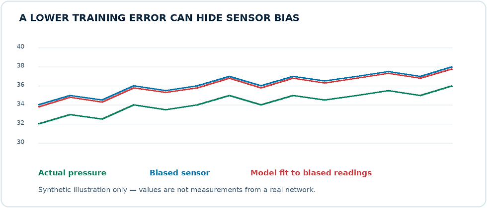
The plotted series are synthetic and demonstrate a possible failure mechanism, not measured results. A credible evaluation needs a trustworthy reference, an appropriate test design, and coverage of relevant locations and operating conditions. Reliability depends on the complete workflow: measurement quality, data alignment, physical assumptions, forecasting, uncertainty handling, and diagnosis.

From prediction to understanding

Return to the initial discrepancy: a forecast of 34.0 m and a measurement of 36.5 m. At first, the only established fact was that the values disagreed. An independent measurement could reveal a sensor problem. Operating records and hydraulic analysis could support a physical explanation. Further investigation could reveal that the forecasting model lacks an important input. Or the available evidence could remain insufficient to choose between the alternatives.

Different evidence leads to different conclusions, and different conclusions lead to different interventions. The model matters, but so do the sensors, physical relationships, assumptions, data pipeline, and diagnostic method that connects them.

When a prediction disagrees with reality, the first task is not to force the two to agree. It is to understand what the disagreement can—and cannot—tell us.

References: U.S. Environmental Protection Agency, EPANET documentation; Vrachimis et al., “Leakage detection and localization in water distribution systems: A model invalidation approach,” Control Engineering Practice (2021), https://doi.org/10.1016/j.conengprac.2021.104755. All numerical values and plotted data in this article are illustrative, not measurements from a real network.